Computation/behind the work

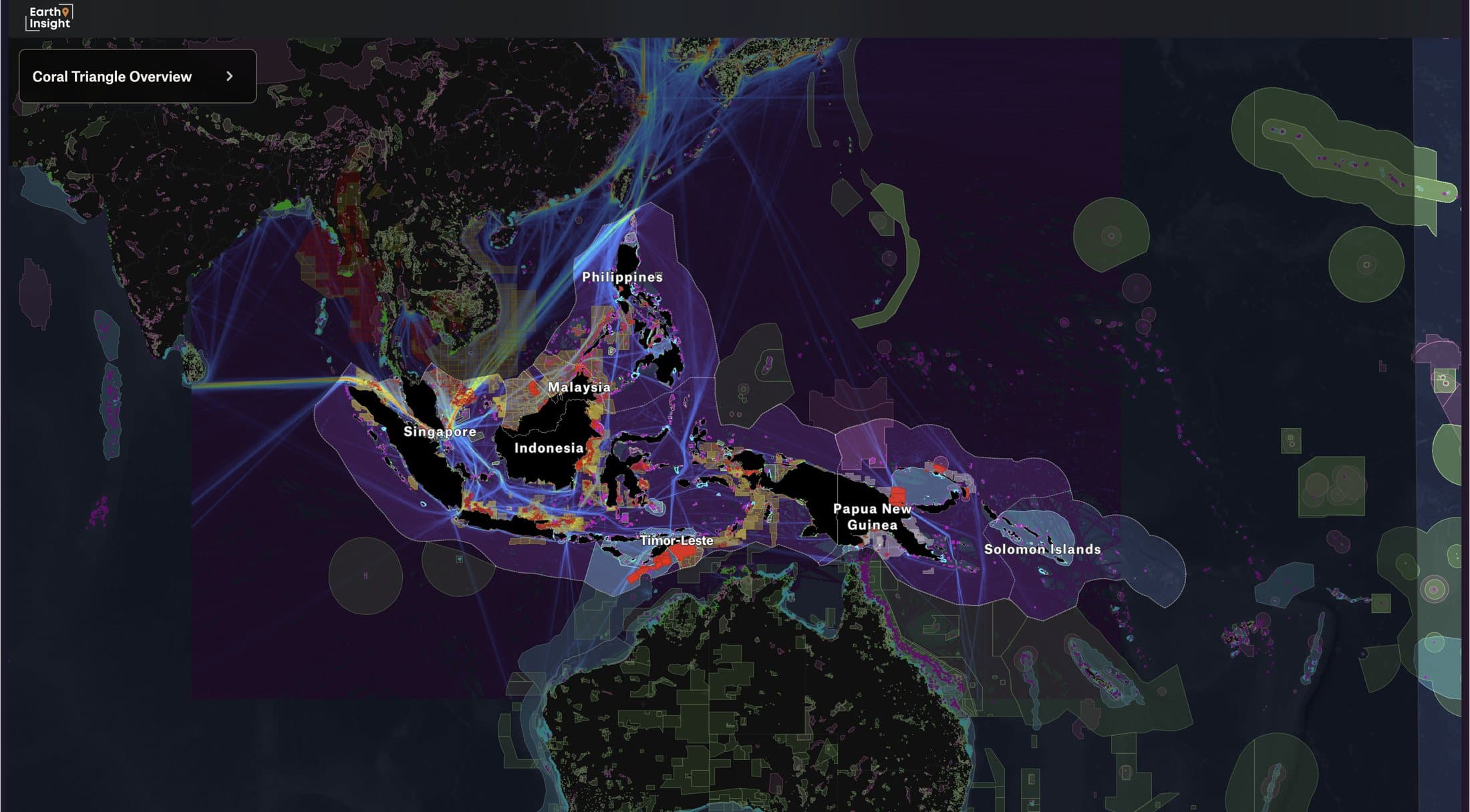
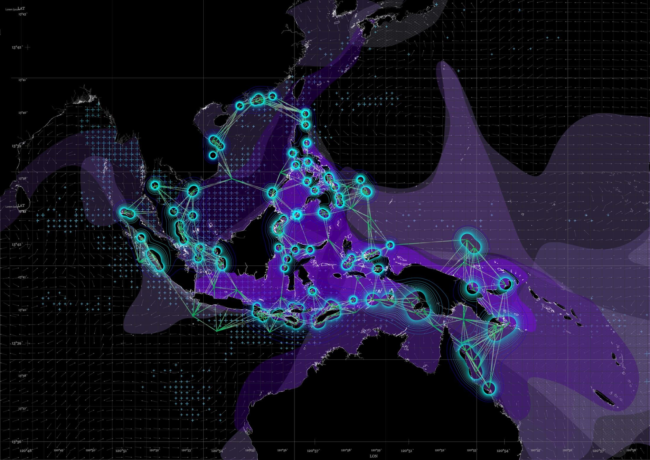
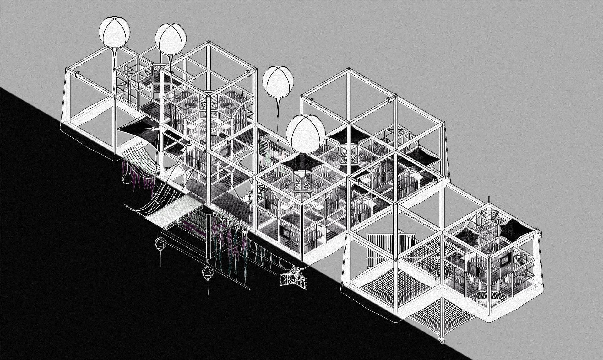
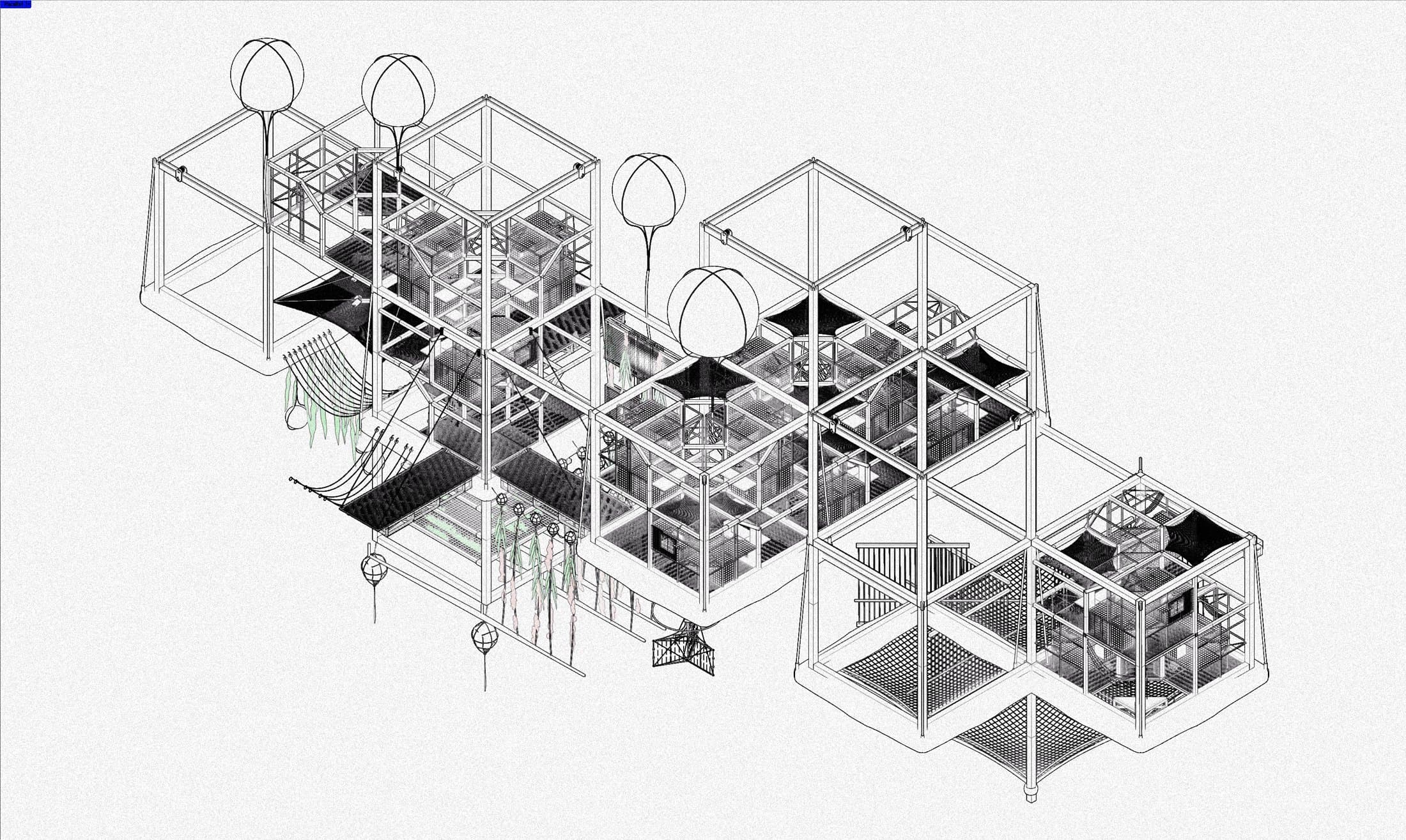
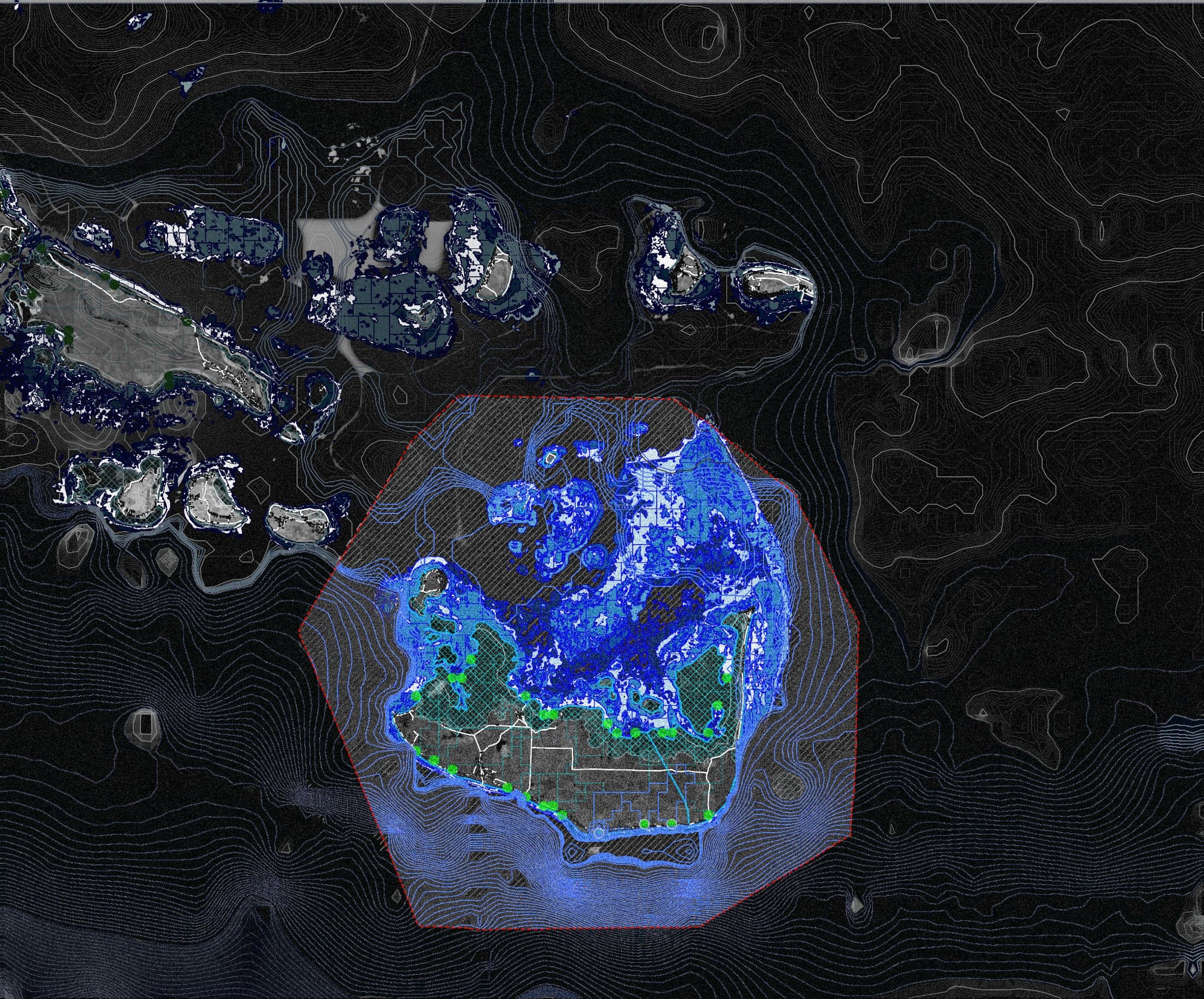
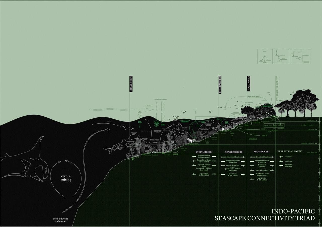
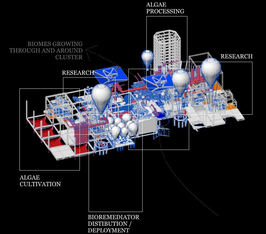
The thesis treats the seascape as a running program. A hexagonal lattice over the Sunda shelf carries a cellular automaton whose rule set grows reef substrate the way coral does — accreting where neighbours already hold, dying back where it is crowded or starved. Technohuman agents move over that lattice, sensing water chemistry, reef signal and fauna, and deciding where to dock, seed or withdraw. Their sensors give non-humans a legible voice, and that voice is counted: a Decentralised Autonomous Commons (a DAO whose members are also reefs, currents and fish) weighs proposals and steers where the floating infrastructure redeploys next.

Lattice. The seascape is discretised as a flat-topped hexagonal grid so every cell has six equidistant neighbours; this avoids the anisotropy of a square Moore neighbourhood, where diagonal growth outruns orthogonal growth. Cell size is set from the bathymetry raster resolution (30 m). Each cell holds a state ∈ {0 water, 1 substrate, 2 coral}, a nutrient scalar read from the current field, and a biodiversity weight from the Coral Triangle GIS layers.

Automaton. The transition function is Life-like but gated: substrate becomes coral when exactly 2 or 3 of its neighbours are coral and the local nutrient value exceeds 0.35; coral persists while it has 2–4 coral neighbours and reverts to substrate outside that band (starvation below, crowding above); water accretes to substrate where three or more substrate neighbours and at least one coral meet. Because nutrient is advected by the current vector field each generation, growth is directional — ridges form across the flow, as they do on real fore-reefs.

Agents. Technohumans are agents with a position on the lattice, a sensing radius of two cells, and a scalar utility U = w₁·coral + w₂·nutrient + w₃·biodiversity − w₄·crowding. Each step an agent evaluates U over its neighbourhood, moves along the steepest ascent, and docks when the gradient falls under a threshold; docked agents raise the local nutrient (growth pods) and register a proposal with the commons. Agents leave when yield decays below a floor for k consecutive steps.

Commons. The Decentralised Autonomous Commons is a weighted-voting DAO whose membership includes non-human actors. Each member m has a weight w(m): for reefs, seagrass and fauna it is 0.6 + 0.4·signal, where signal is the normalised sensor reading that member represents; for human members it is 0.5·min(1, credit). A proposal passes when Σ w(m) over supporting members ÷ Σ w(m) over all members ≥ 0.55. The decision writes to a ledger that the geometry layer reads: pass → redeploy pods to the proposal's target cells; fail → hold. The effect is that a bleaching reef, whose signal is high, out-votes a marina whose credit is high but capped.

#cellularautomata#agentbased#DAO#morethanhuman#GIS

EcoTwin is the agent layer of the thesis made executable: a habitat digital twin of the Pasir Ris intertidal zone. Every agent is one mangrove — a propagule that drifts on the tide, settles where suitability is high, grows, competes for light with its neighbours and reproduces. Suitability is a product of Gaussian responses to inundation and salinity, tuned per species from field literature; the tide itself is reconstructed from Singapore's harmonic constituents. It is the same sense → decide → act loop the technohumans run in the manifesto, here calibrated against real species.

State. Each agent carries position (x along shore, y cross-shore in metres), species, stage ∈ {propagule, established}, age, height, canopy radius, health and a competition score. The world is 500 × 220 m with a sea edge at y = 70, upper intertidal at 160 and land from 165.

Environment. Water level h(t) = MSL + Σ Aᵢ cos(ωᵢ t) over the four principal constituents M2 (0.80 m, 28.984°/h), S2 (0.32, 30.000), K1 (0.14, 15.041) and O1 (0.10, 13.943), MSL 1.25 m above chart datum. Inundation fraction per cross-shore position is integrated from h(t) over a lunar day; salinity is a landward gradient with alongshore noise.

Suitability. s = exp(−½((I−μ_I)/σ_I)²) · exp(−½((S−μ_S)/σ_S)²) · (1 − 0.6·c), where I is inundation, S salinity and c the competition score; μ and σ are species constants from Komiyama et al. (2008), Friess & Webb (2014), Richards & Friess (2016) and Duke (2001).

Dynamics. Propagules advect with a random drift plus a tidal term and settle if inside the intertidal band with s > 0.5. Established trees grow by g = baseGrowth · s per day to a species maximum; canopy = height · canopyRatio. Competition is c = min(1, Σ_j canopy_j / (d_ij² + 0.1) / 8) over neighbours within canopy + 1 m — an O(n²) kernel, acceptable for n ≲ 1 000. Mortality when s < survivalFloor or health ≤ 0; reproduction after reproductionAge, releasing propagules within dispersalRadius.

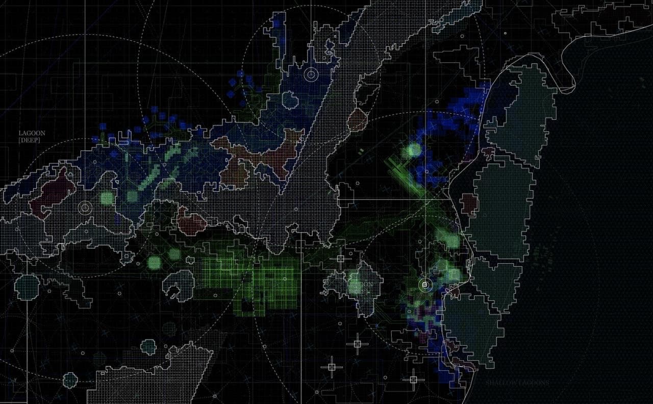
Output. A flat-topped hex planning grid (22 m radius) is laid over the domain and coloured by occupancy per species, so the run can be read like a Marxan solution and exported as GeoJSON for restoration planning.

#agentbased#digitaltwin#mangrove#restoration

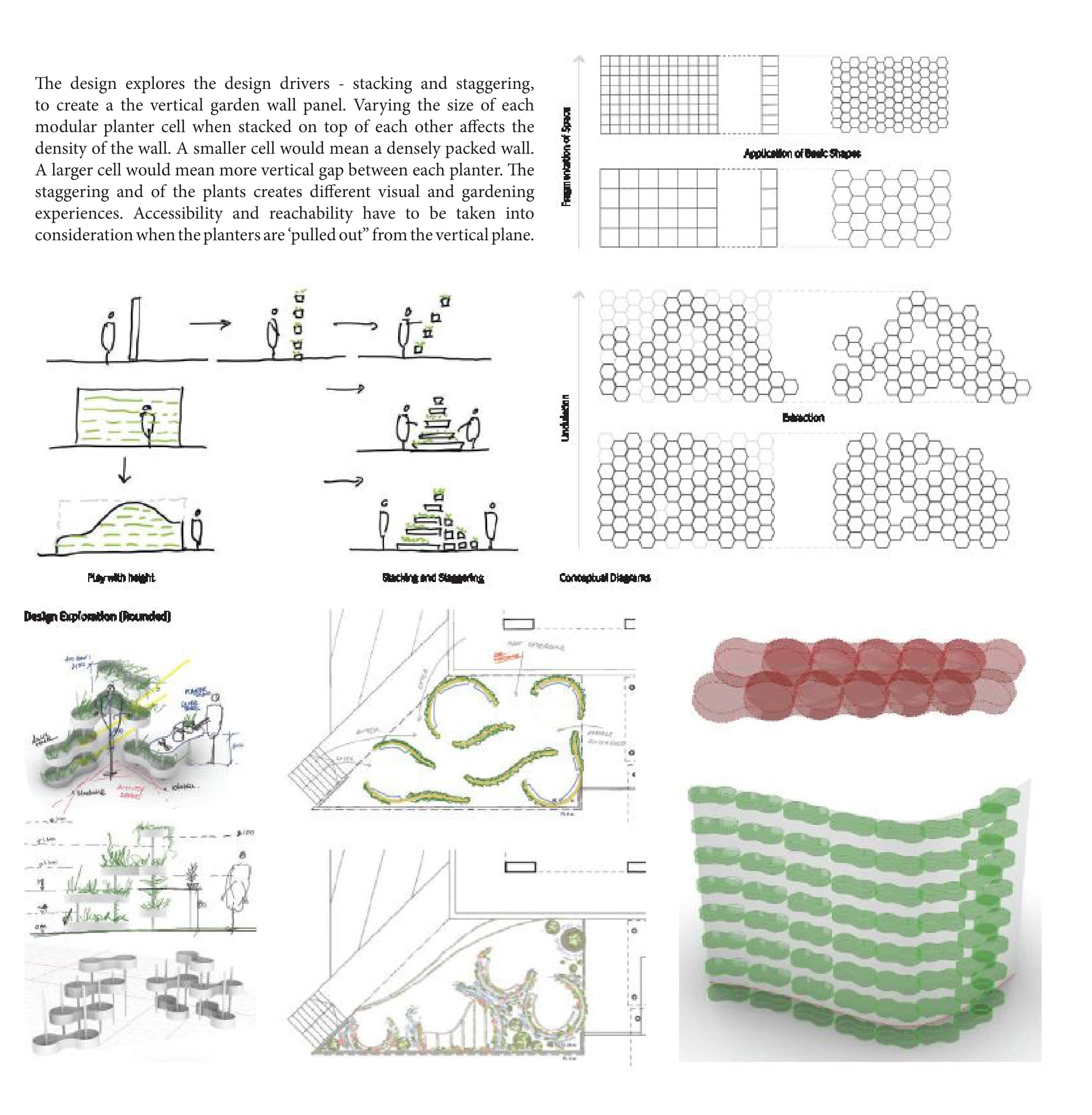
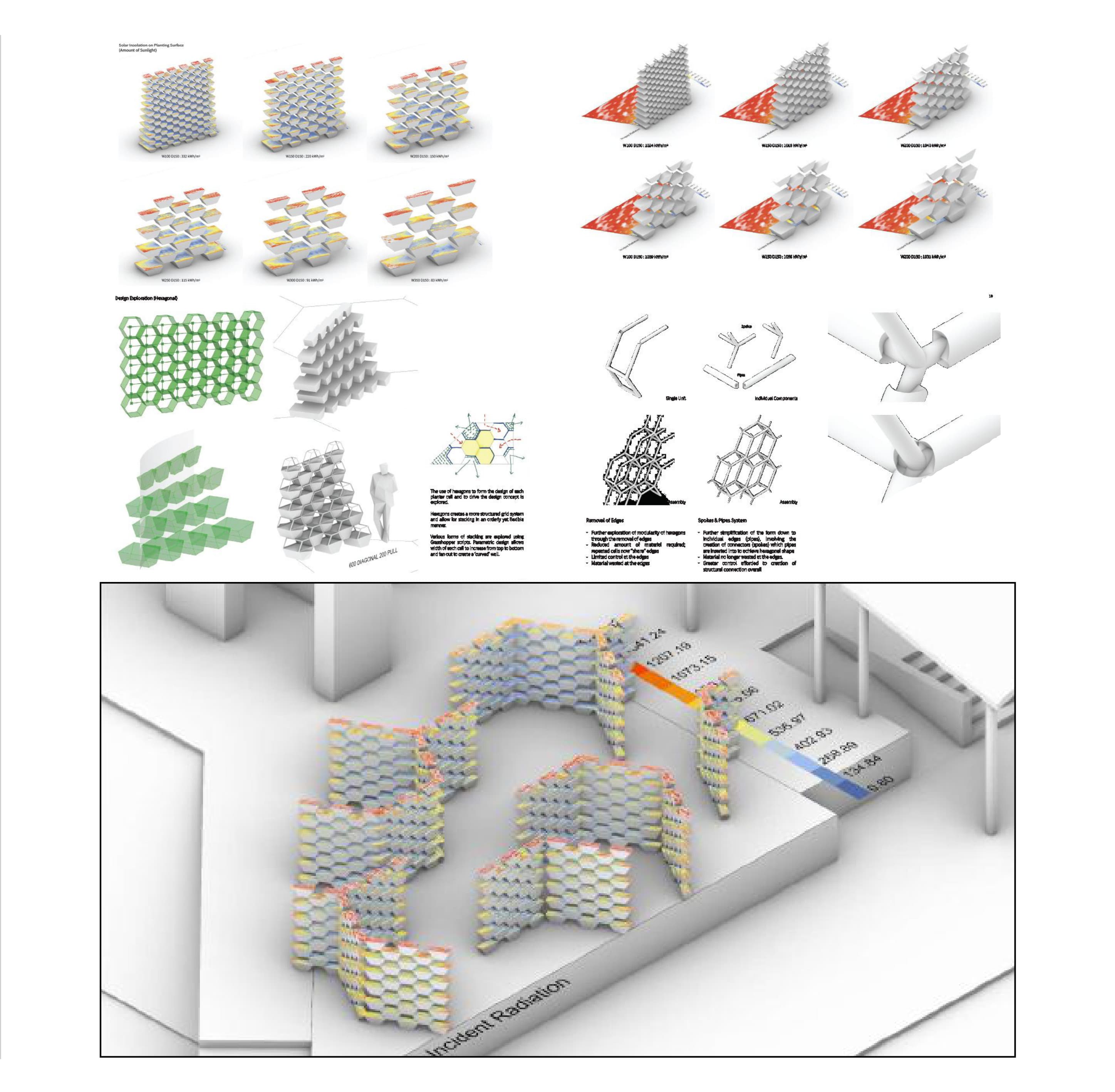
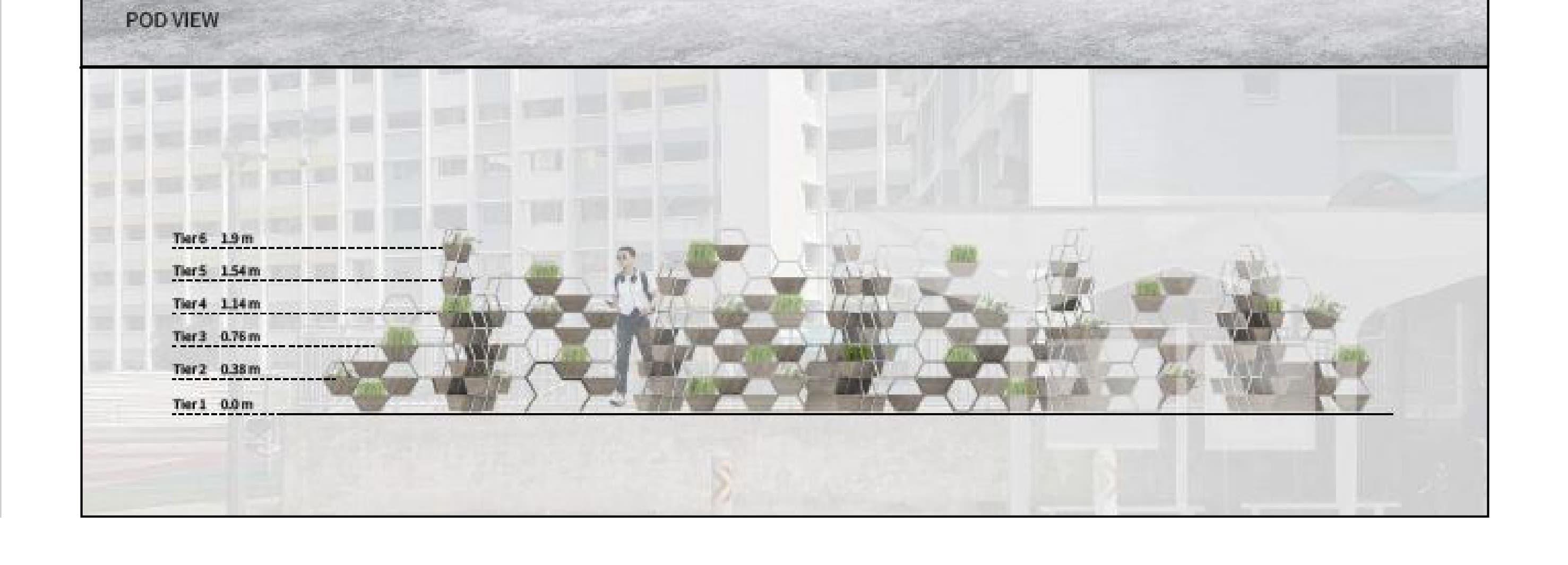
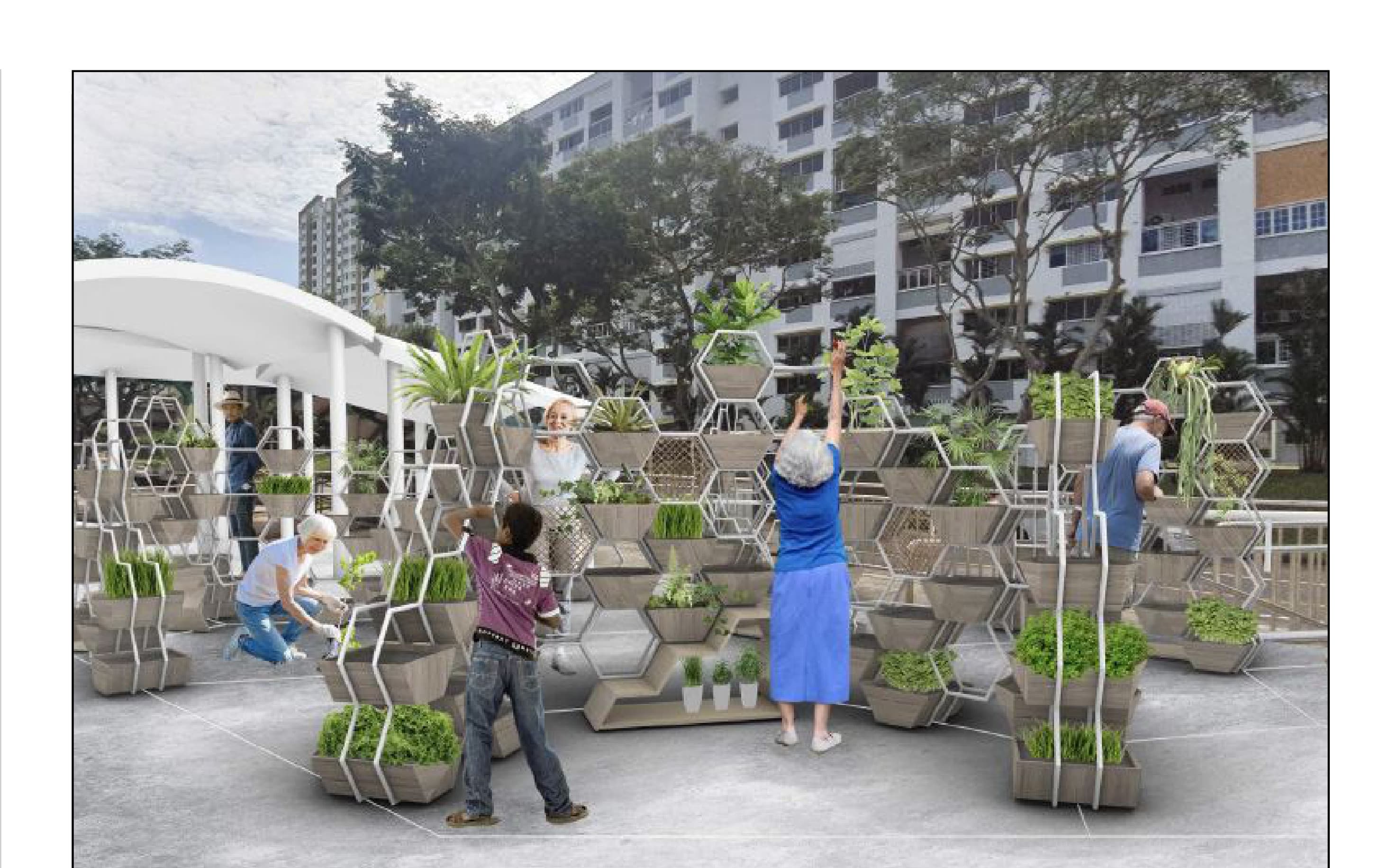
Cell Wall is a single parametric definition. A hexagonal grid is laid over the site; each cell's size is remapped from its distance to the circulation spine, so the wall densifies where people gather and opens where it should breathe. A cull pattern staggers the planters, and a tier vector pulls them off the vertical plane in steps from 0.0 to 1.9 m. A small script then checks every cell against reach envelopes — standing, seated, wheelchair — and flags the ones a resident could not tend, which drives the next iteration.

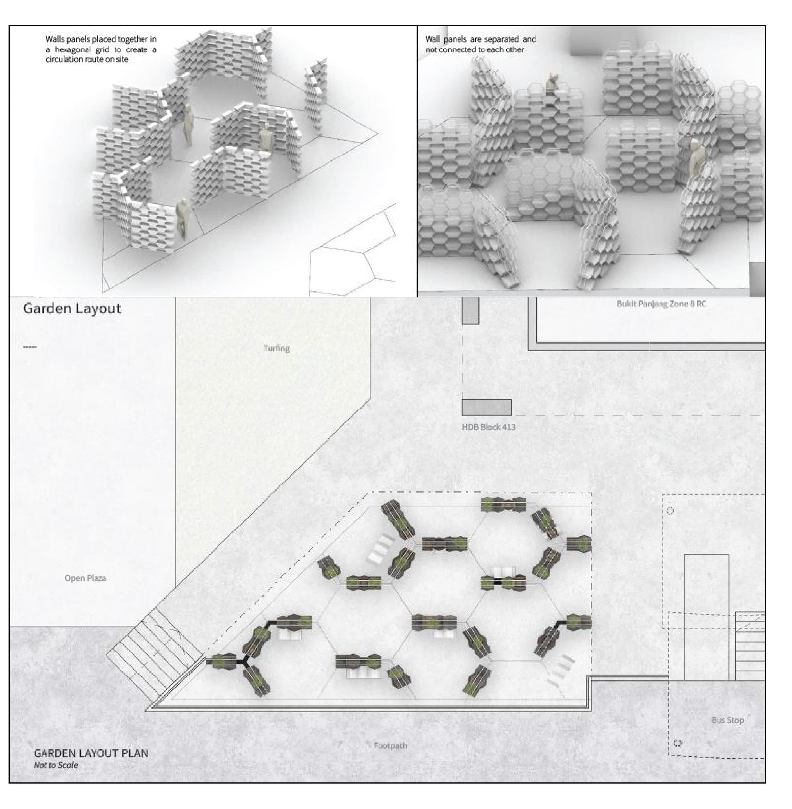
Grid. A flat-topped hexagonal grid is generated over the site boundary; cell centroids are the design variables. A curve drawn along the intended circulation acts as the attractor.

Density. For each centroid, d = distance to the attractor curve; cell size = remap(d, [d_min, d_max] → [0.90, 0.45] m). Distance is inverted so cells shrink and pack tightly near the spine and open up away from it; this both reads as a gradient and concentrates planting where people pass.

Stagger and tiers. A cull pattern (T, F, T) staggers alternate cells; the survivors are moved out of the wall plane by a vector whose length steps through 0.0 → 0.4 → 0.8 → 1.2 → 1.6 → 1.9 m by row, so the planters form terraces rather than a flat face.

Reach check. A GhPython component takes the planter breps and a user type and classifies each by centroid height against an envelope: wheelchair 0.4–1.2 m, seated 0.4–1.4 m, standing 0.5–1.9 m. The failing set is reported back as a count and as geometry, and the attractor / tier vector are adjusted until every tier is tendable by at least one user type and the lowest tier by all three.

#grasshopper#hexgrid#attractor#accessibility

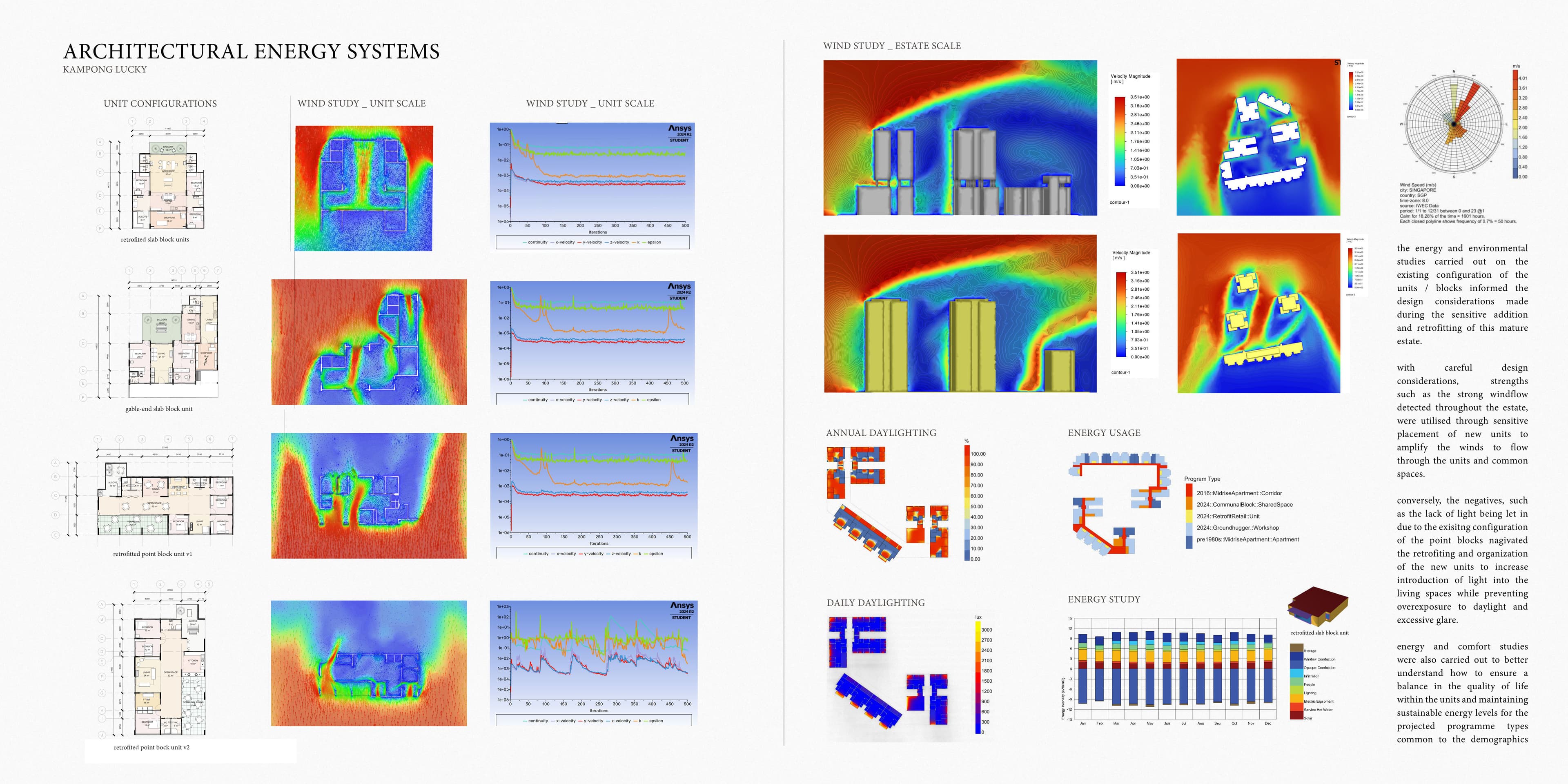
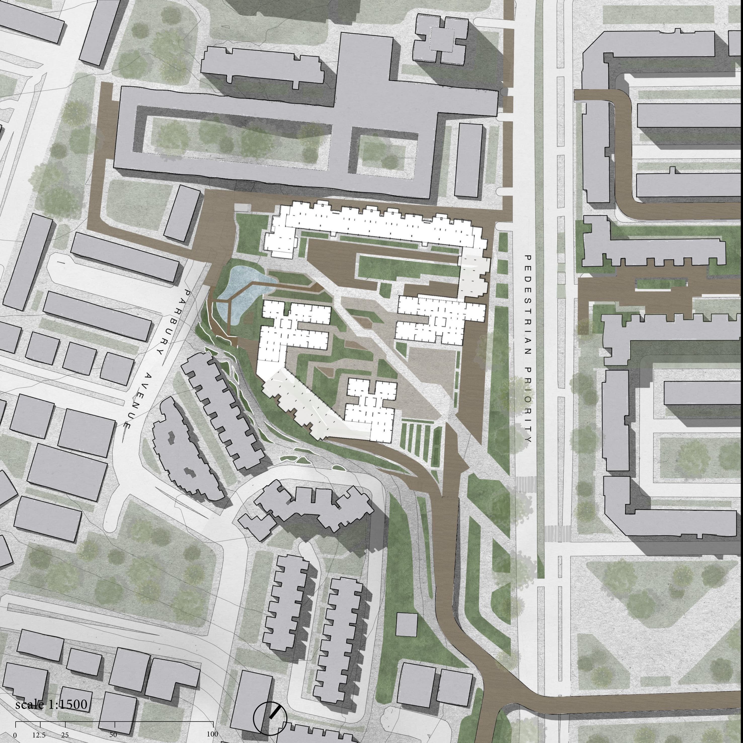
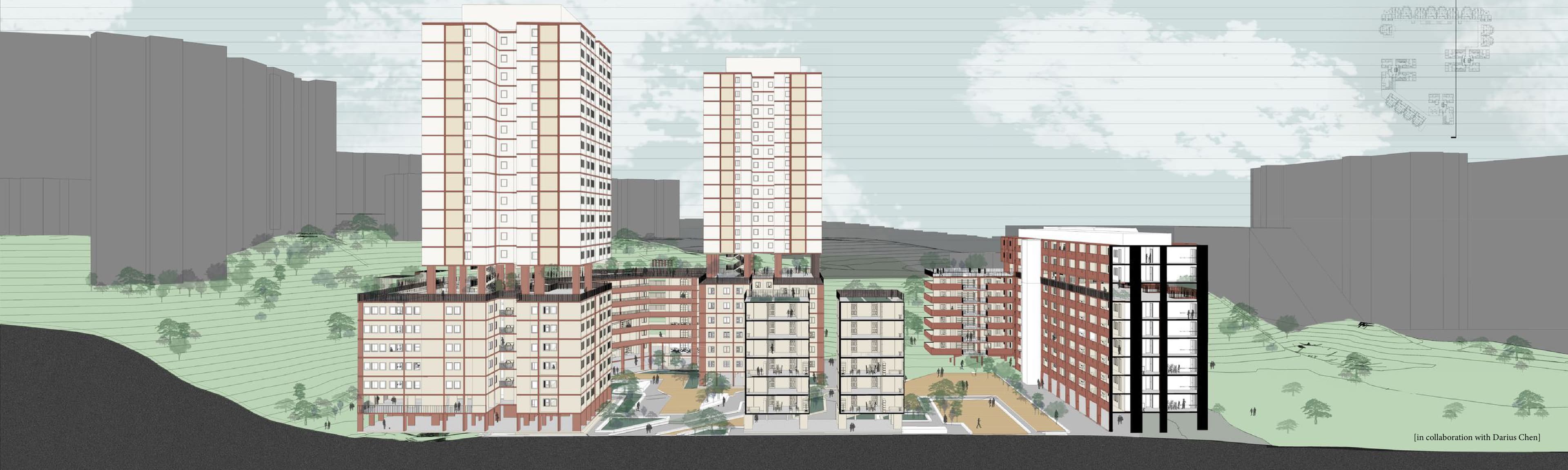
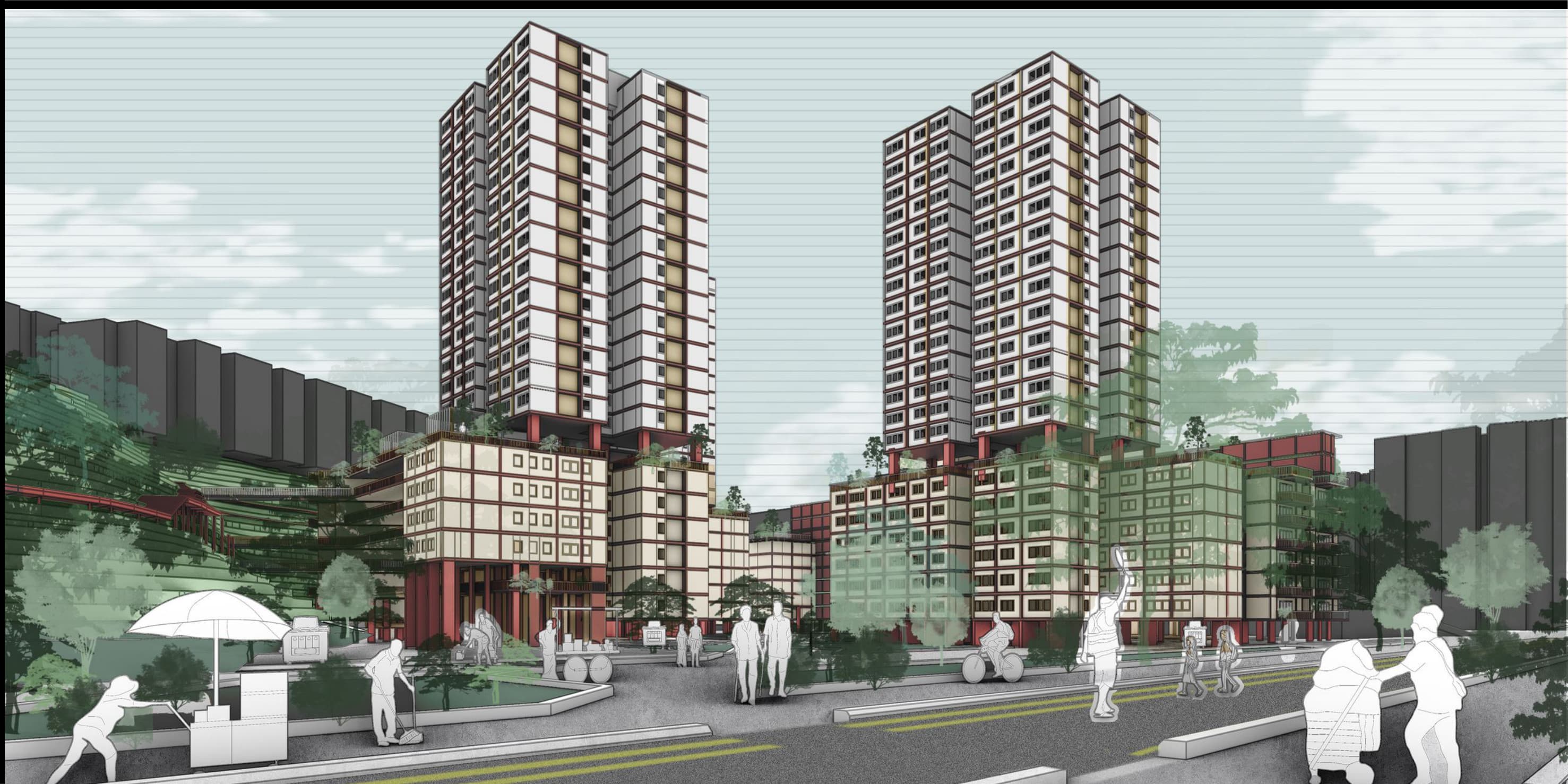
Kampong Lucky's massing was tuned by simulation. A structured Cartesian mesh around the estate is solved with a RANS k-ω SST model for the two monsoon directions; radiation is run alongside; both are folded into a comfort index and a genetic optimiser moves the void-deck cuts, verandah depths and block offsets until the courtyards sit in the comfortable band. The solver is the same one behind webCFD — a PIMPLE-style incompressible Navier–Stokes solver with VOF free-surface tracking, written in TypeScript.

Domain. The estate blocks are meshed into a structured Cartesian grid Nx × Ny × Nz with cells refined near the void decks; the domain extends five block heights upstream and fifteen downstream so the wake resolves before the outlet. Inflow is a logarithmic boundary-layer profile fitted to the Changi EPW wind rose for the north-east and south-west monsoon cases.

Solver. Incompressible RANS with the k-ω SST closure (σ_k1 0.85, σ_ω1 0.5, β1 0.075, β* 0.09, a1 0.31, κ 0.41), pressure–velocity coupling by the PIMPLE algorithm (PISO inner loop, SIMPLE outer), VOF for the free surface where water is present. Convergence when normalised residuals of p and u fall below 1e-4 and the courtyard probe speed changes by less than 1 % between iterations.

Comfort. Solar radiation on façades and courtyards from Ladybug/Honeybee for the same hours; the UTCI-style index combines wind speed at 1.5 m, air temperature, humidity and mean radiant temperature. The objective is the count of daylight hours in the 26–30 °C comfortable band over the courtyards.

Optimisation. A Galapagos genetic run with a genome of block offsets (±3 m), void-deck cut heights (2.4–4.8 m) and verandah depths (1.2–3.0 m); population 40, twelve generations, elitism 5 %. The best individual opened the ground plane on the windward blocks and deepened the leeward verandahs — which is the massing that was drawn.

#CFD#RANS#ladybug#galapagos#comfort

Memorium is carved from the canyon by a sequence rather than a plan. The emotional arc — fear, anxiety, heaviness, then calm, serenity, the sublime — is drawn as graph-mapper curves for light and enclosure; those values drive the boolean carve along a shortest walk through the terrain, so each hall's aperture and volume follow the feeling it is meant to hold. Sun-path and a Sabine reverb estimate check each chamber: the deprivation rooms are held under 0.3 s RT60, the Final Act Hall opens to the sky.

Path. A shortest walk is computed over the canyon digital elevation model between the hospice and the Final Act Hall, with slope penalised above 1 : 12 so the procession stays accessible; the walk is divided into six stations, one per emotional state.

Envelopes. Two graph mappers turn the sequence into scalar fields along the path: light L(t) rises from 0.08 at the deprivation chambers to 1.0 at the Final Act Hall; enclosure E(t) falls from 1.0 to 0.1. At each station the hall's aperture area is proportional to L and its plan depth to E, so form is read off the curves rather than composed.

Carve. The halls are subtracted from the terrain solid by boolean difference; walls are offset inward by the enclosure value so the deprivation rooms are thick-walled and the last hall almost open.

Checks. Ladybug sun path at the equinox confirms the aperture of each hall receives the intended light; a C# component estimates reverberation by Sabine, RT60 = 0.161·V / Σ α·S, with absorption coefficients for canyon stone and the felt linings, and holds the deprivation chambers below 0.3 s.

#graphmapper#boolean#ladybug#acoustics